Statistics

Measures of Center

• Suppose we have observations `y_1, ..., y_n`

• mean: `bar(y) = (y_1 + ... + y_n)/n = 1/n sum_(i = 1)^n y_i`

• median:

• - arrange numbers in increasing order

• - if `n` is odd, the median is the observation in center

• - if `n` is even, the median is the mean of the two observations in the center

• Note: mean is greatly affected by outliers (unusual values) while median is robust (not sensitive to outliers)

Measures of Variation

• variance: `s^2 = 1/(n-1) sum_(i = 1)^n (y_i - bar(y))^2`

• standard deviation: `s` (square root of variation)

• interquartile range (IQR):

• - arrange data in increasing order

• - lower quartile `Q_1` is the median of the observations to the left of the median

• - upper quartile `Q_3` is the median of the observations to the right of the median

• - IQR = `Q_3 - Q_1`

• Note: standard deviation is sensitive to outliers. IQR is not.

• Use the mean and standard deviation if the data is symmetric and there are no outliers

• Use the median and IQR if the data is skewed and there are outliers

Relative Standing

• Suppose we have observations `y_1, ..., y_n`

• z-score: number of standard deviations away from the mean

• To find the z-score associated with a given `y_i`, subtract the mean of the observations and divide by the standard deviation

• `z = (y_i - bar(y))/s`

Changes in Scale

• Suppose `x_i = a + by_i`, `b > 0`, for `i = 1, ..., n`

• Then `bar(x) = a + b bar(y)`

• And `s_x` (standard deviation of x) ` = bs_y`

• And z-score = `(x_i - bar(x))/s_x = ((a+by_i)-(a+b bar(y)))/(bs_y) = (y_i - bar(y))/s_y`

• In words: change each observation `y_i` by some amount (by adding and/or multiplying each `y_i` by some value(s))

• - Finding the mean of the changed values is the same as applying the changes to the mean of the old values

• - The standard deviation is unaffected by addition, but finding the standard deviation of the changed values is the same as multiplying the old standard by the amount multiplied to each `y_i`

• - The z-score is unaffected by changes in scale

Correlation

• A measure of linear association between two quantitative variables

• Suppose we have two variables `x` and `y` whose values for `n` cases are `(x_1, y_1), ..., (x_n, y_n)`

• Let `bar(x)` and `bar(y)` be means, let `s_x` and `s_y` be standard deviations

• The correlation between `x` and `y` is `r = 1/(n-1) sum_(i = 1)^n ((x_i-bar(x))/(s_x))((y_i-bar(y))/(s_y))`

• If `x` and `y` are positively associated (large values of `x` are paired with large values of `y`) then `r > 0`

• If `x` and `y` are negatively associated (large values of `x` are paired with small values of `y`) then `r < 0`

• If `x_i = y_i` for all `i`, then `r = 1/(n-1) sum_(i = 1)^n (x_i-bar(x))^2/(s_x)^2 = (s_x)^2/(s_x)^2 = 1`

• If `x_i = -y_i` for all `i`, then `r = -1`

• We always have `-1 <= r <= 1`

• Correlation is unaffected by changes in scale

Linear Regression

• Goal: predict the value of a variable `y` (response variable) given the value of a variable `x` (explanatory variable)

• Fit a line to the data and use the line to predict `y` from `x`

• Equation of the line is `hat(y) = b_0 + b_1x` where `b_0` is the intercept and `b_1` is the slope



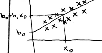
• If the value of the explanatory variable is `x_0` then the prediction for the response variable is `b_0 + b_1x_0`

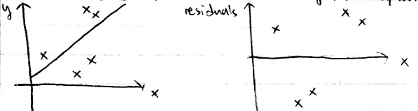
• For each point, the vertical distance `y-hat(y)` between the point and the line is called the prediction error or residual

• least squares regression line: the line that minimizes the sum of squares of residuals

• Let `bar(x)` and `bar(y)` be the means of two variables

• Let `s_x` and `s_y` be the standard deviations

• Let `r` be the correlation

• The least squares regression line is `hat(y) = b_0 + b_1x` where `b_1 = (rs_y)/s_x` and `b_0 = bar(y) - b_1bar(x)`

• The intercept (`b_0`) often has little statistical meaning

• If the regression line goes through `(bar(x), bar(y))`, then if `x` is the average, then `y` is also the average

• If `x = bar(x)+s_x`, then `hat(y) = b_0 + b_1(bar(x)+s_x) = b_0 + b_1bar(x) + b_1s_x = hat(y) + rs_y`

• In words, if `x` is one standard deviation above the mean, we predict `y` to be `r` standard deviations above the mean

• Because `-1 <= r <= 1`, this leads to the "regression effect"

Assessing the Appropriateness of Regression

• residual plot: a plot of residuals against the explanatory variable



• If the residual plot looks like a random scatter with no apparent pattern, then the regression line is a good representation of the relationship between the variables

• - About 50% above and below

• Things to look for:

• - curvature

• - outliers (large residuals or points that are extreme in the `x`-direction

• - heteroskedasticity (uneven spread)



• Low values of `x` have a small spread while large values of `x` have a larger spread

• If there is curvature or extreme heteroskedasticity, try a transformation

• Replace `y` by `y^2` or `sqrt(y)` or `1/y` or logs of one or both variables

• A point has high leverage if it is extreme in the `x`-direction

• A point is influential if omitting it would greatly change the slope of the line

Assessing the Quality of Fit

• The fraction of the variation in `y` explained by the regression is called `R^2` and it is the square of the correlation

• If `R^2` is high, regression could be inappropriate if there is a way of getting better predictions



• Could do better by not using a line because the points are curved

• If `R^2` is low, regression could be appropriate if there is no way to do better