Advanced Artificial Intelligence
Shortcut to this page: ntrllog.netlify.app/ai2
Notes provided by Professor Armando Beltran (CSULA), Introduction to Evolutionary Computing, and Build a Large Language Model (From Scratch)
This is an extension of the artificial intelligence and machine learning resources. Well, we’ll see where this goes — I’m writing this as the class goes.
What's the Problem?
As computer scientists, we aim to develop and use AI to solve problems optimally. But before we look at how AI works, we should start with understanding what types of problems exist and how to define them.
Black Box Model
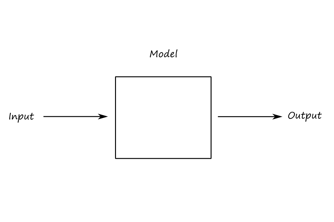
Some problems can be reduced to a "black box" model. The "black box" model has `3` components: an input, a model (algorithm or function), and an output. If one of the three components is unknown, then that is a problem we can define and solve.
Optimization
If the input is unknown, then we have an optimization problem. As the name implies, optimization problems seek to maximize or minimize a result.
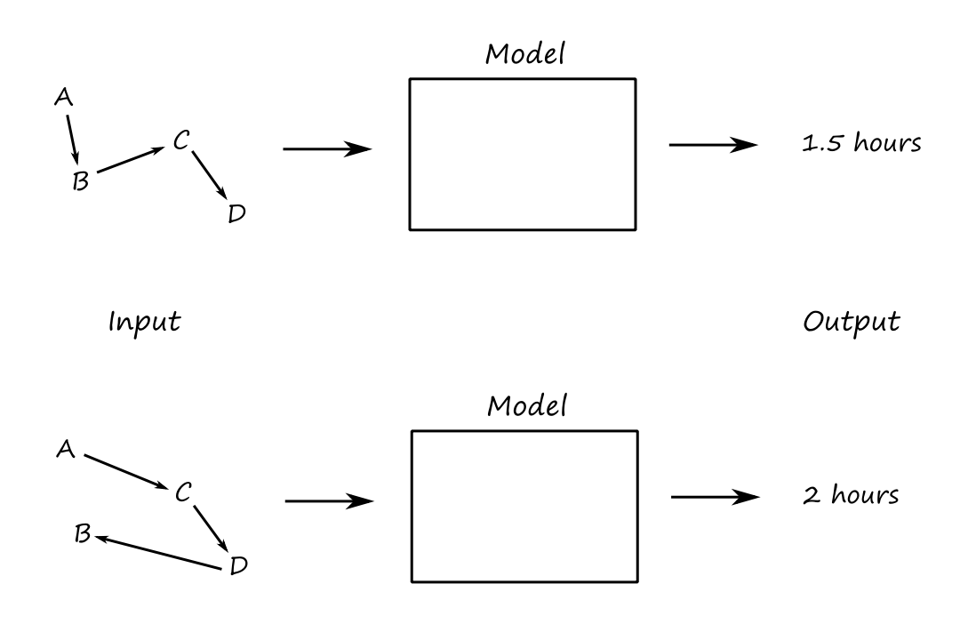
For example, we’re traveling and we want to visit a bunch of destinations while minimizing time traveled, i.e., we want an efficient route so that we don’t waste time. The model is a function that calculates the time it takes to go from one destination to another. The output is a number representing the total time traveled (we want to minimize this). The input — which is what we want to solve for — is a route.
Another example is the `8`-queens problem. We want to place `8` queens such that no queens are attacking each other. The model is a function that calculates how many queens are attacking each other. The output is the number of queens attacking each other (we want to maximize this). The input — which is what we want to solve for — is a configuration of `8` queens.
Objective Function
As mentioned earlier, optimization problems aim to maximize or minimize a result. That result is calculated by a function, namely an objective function. An objective function is a math expression that quantifies the quality of a potential solution to an optimization problem. (The quality of a solution is how well it solves the problem.)
In other words, an objective function assigns a numerical value to an input, and that numerical value is a measure of how good that input is as a solution to the problem.
Modeling
If the model is unknown, then we have a modeling problem. In these types of problems, we have the inputs and outputs, and we want to know what type of model fits the data.
Let’s say we have these inputs and outputs:
| x | y |
|---|---|
| `1` | `2` |
| `2` | `4` |
| `3` | `6` |
| `4` | `8` |
| `5` | `10` |
In this case, we can figure out that the model is the function `y = 2x`.
A real-world example is voice recognition. We have the inputs (a set of spoken text) and the outputs (a set of written text), and we want to build a model that can match the spoken text to the written text.
Modeling problems can be transformed into optimization problems by picking a model that works and then optimizing that model.
Simulation
If the output is unknown, then we have a simulation problem. These types of problems are like exploring "what if" scenarios.
For example, predicting the weather is a simulation problem. The inputs are data points for things like humidity and temperature. The model is a function that takes in those data points and returns a weather. "What if it is humid and hot?"
The Search for Answers
Honestly, simulation problems don’t really sound like "problems" at all. All we need to do is run the model on the inputs and get our answer.
On the other hand, for optimization and modeling problems, we have to search for something. For optimization problems, we have to find the input that gives us the desired output. For modeling problems, we have to find the model that gives us the desired output for the given inputs.
Formally, there is a search space, which is a set of objects of interest, including the desired solution. It can typically be represented as a search tree.
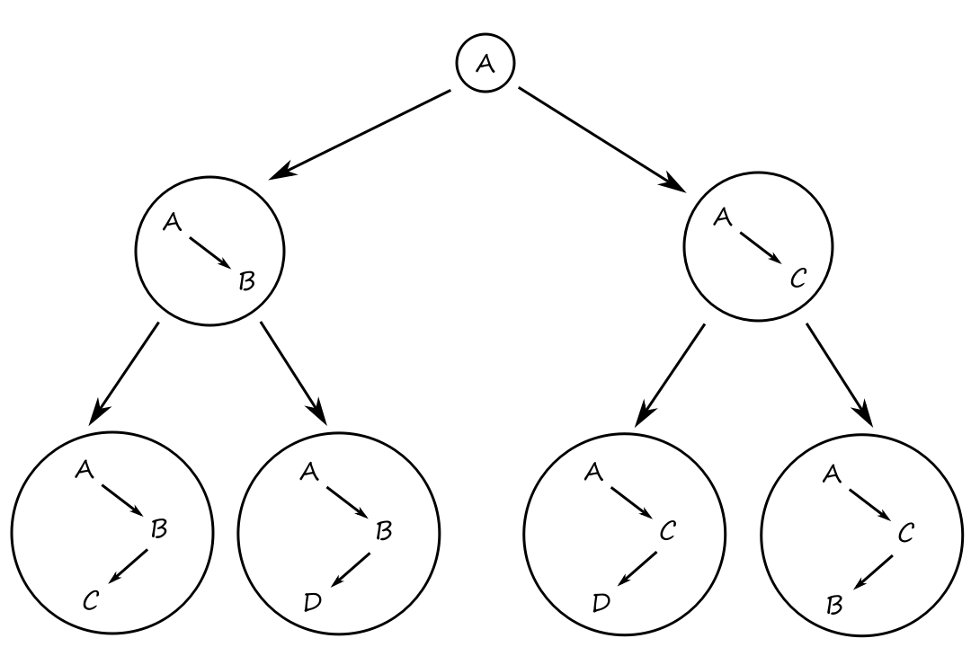
For the time-efficient traveling problem, the search space is a bunch of possible routes and we have to find one that is the most time-efficient. For the voice-recognition problem, the search space is a bunch of models and we have to find one that is the most accurate.
Typically, the search space for any problem will be very large, so we need an efficient way to explore the search space for the desired solution. A problem solver does this for us. A good problem solver goes through the search space and finds the optimal path through the search tree to the desired solution.
NP Problems
Some problems are inherently hard for computers to solve. This could be because it takes a really long time and/or a lot of memory is needed to find the solution. The difficulty of a problem can be classified into four categories:
- Class P: problems that can be solved in polynomial time
- Class NP: problems that can be verified in polynomial time
- the "N" stands for "nondeterministic"
- Class NP-complete: a problem `p` is NP-complete if every other NP problem can be transformed/reduced to `p`
- if it turns out that an NP-complete problem can be solved in polynomial time, then all NP problems can be solved in polynomial time
- Class NP-hard: problems that are at least as hard as NP-complete problems, but the solution may not be verfiable in polynomial time
These classifications (except for NP-hard) apply to decision problems: problems that have a "yes" or "no" answer. For example, "Is `A rarr B rarr C rarr D` the optimal route?"
The `n`-Queens Problem
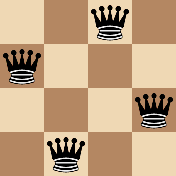
The `n`-queens problem is an optimization problem that involves placing `n` queens on a chessboard such that none of the queens are attacking each other. For example, for `n=4`:
To formalize things, we can frame the problem statement as, "Given `n` queens, find a configuration for the queens on an `n xx n` chessboard that maximizes the number of pairs of non-attacking queens."
If we label the top-left corner as row `1`, column `1`, then we can represent a board configuration using coordinates. So for the example above, we have
`Q = {(2,1), (4,2), (1,3), (3,4)}`
The objective function `f` can be represented as
`max_Q f(Q) = (n(n-1))/2-A(Q)`
where `A(Q)` is the number of pairs of attacking queens for a board configuration `Q`.
`A(Q)` is the number of pairs of attacking queens (as opposed to the number of queens being attacked). In this example, there are `4` pairs of attacking queens.
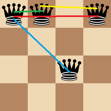
`(n(n-1))/2` is the number of total possible pairs of queens. If we subtract the number of pairs of attacking queens from that expression, we get the number of pairs of non-attacking queens (which is what we're trying to maximize).
Free Optimization Approach
Now that we have formally defined the problem, we can start to look at how hard this problem is to solve. For optimization problems, the difficulty depends on the size of the search space. The more inputs there are to search through, the harder the problem is.
So how many possible board configurations are there? We'll first consider the `n=4` case.
For the first queen, there are `16` spaces for where it can be placed. For the second queen, there are `15` spaces. For the third queen, there are `14` spaces. For the last queen, there are `13` spaces. So there are a total of `16*15*14*13=43,680` possible board configurations.
In general, there are
`(n^2!)/((n^2-n)!)`
possible board configurations.
For a standard `8xx8` chessboard, there are `1.78 xx 10^(14)` possible board configurations. Yeah, that's a lot to search through.
Constrained Optimization Approach: Row Constraint
Is it possible to make the search space smaller? Well, notice that if more than `1` queen is on the same row, then they're automatically attacking each other.
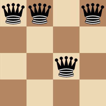
So any board configurations where there is more than `1` queen in the same row can be removed from the search space. We can achieve this by reframing the problem statement as, "Given `n` queens, find a configuration for the queens on an `n xx n` chessboard such that every row contains exactly one queen while maximizing the number of pairs of non-attacking queens." We're introducing a constraint on the original problem.
Also, instead of using coordinates to represent a board configuration, we can use a vector representation.
`Q = [Q_1, Q_2, ..., Q_n]^T`
where index `i` represents the row number and `Q_i` is the column number.

`Q = [3, 1, 4, 2]^T`
By using a vector, we force all possible board configurations to have exactly `1` queen in every row.
Let's see how much the search space has been reduced by with this new constraint. Again, we'll first consider the `n=4` case.
The first queen can only be placed in the first row, and in the first row, there are only `4` spaces for it. The second queen can only be placed in the second row, and in the second row, there are only `4` spaces for it. The third queen can only be placed in the third row, and in the third row, there are only `4` spaces for it. The last queen can only be placed in the fourth row, and in the fourth row, there are only `4` spaces for it. So there are a total of `4*4*4*4=256` possible board configurations.
In general, there are
`n^n`
possible board configurations.
So we went from `43,680` to `256`, which is pretty good. For the `n=8` case, there are `16,777,216` possible board configurations, which is much less than `1.78 xx 10^(14)`, but still a lot.
Constrained Optimization Approach: Row and Column Constraint
We can apply the same row-constraint reasoning to the columns as well: if there is more than `1` queen on the same column, then they're automatically attacking each other.
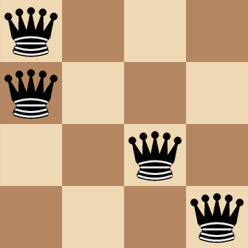
So any board configurations where there is more than `1` queen in the same row and column can be removed from the search space. We can achieve this by introducing another constraint: "Given `n` queens, find a configuration for the queens on an `n xx n` chessboard such that every row and column contains exactly one queen while maximizing the number of pairs of non-attacking queens."
Mathematically, for all `1 le i,j le n`, `Q_i != Q_j` and `i != j`.
Let's see how much the search space has been reduced by with this new constraint. Again, we'll first consider the `n=4` case.
The first queen can only be placed in the first row, and in the first row, there are only `4` spaces for it. The second queen can only be placed in the second row, and in the second row, there are only `3` spaces for it. The third queen can only be placed in the third row, and in the third row, there are only `2` spaces for it. The last queen can only be placed in the fourth row, and in the fourth row, there is only `1` space for it. So there are a total of `4*3*2*1=24` possible board configurations.
In general, there are
`n!`
possible board configurations.
For the `n=8` case, there are now only `4032` board configurations in the search space.
Introducing constraints on the problem made the `n`-queens problem much easier to solve. However, even with the constraints, it is still a hard problem to solve, especially when `n` gets larger. Here's a table with the size of the search space for each version of the problem.
| `n` | free optimization | `1` queen per row | `1` queen per row and column |
|---|---|---|---|
| `4` | `43680` | `256` | `24` |
| `8` | `1.78643 xx 10^14` | `16777216` | `40320` |
| `16` | `2.10876 xx 10^38` | `1.84467 xx 10^19` | `2.09228 xx 10^13` |
| `32` | `1.30932 xx 10^96` | `1.4615 xx 10^48` | `2.63131 xx 10^35` |
| `64` | `9.4661 xx 10^230` | `3.9402 xx 10^115` | `1.26887 xx 10^89` |
So why are we even looking at the `n`-queens problem in the first place? It looks like a trivial puzzle.
Well, it turns out that the `n`-queens problem has practical applications in things like task scheduling and computer resource management.
Evolutionary Computing
Going through each possible board configuration to find a valid one is not practical. It would be better to programmatically generate solutions.
One way of doing this is through evolutionary computing. Evolutionary computing is a research area within computer science that draws inspiration from evolution and natural selection.
Nature is apparently a good source of inspiration. The best problem solver known in nature is the human brain (basis of neurocomputing) and the evolutionary mechanism that created the human brain (basis of evolutionary computing).
The metaphor here is that the problem is like the environment; a candidate solution is like an individual; and the quality of the candidate solution is like the individual's "fitness" level.
The population consists of candidate solutions and the best ones are selected for "reproduction". This produces new solutions (containing the traits from both of the parents), and those new solutions are modified slightly to maintain diversity. And this process repeats.
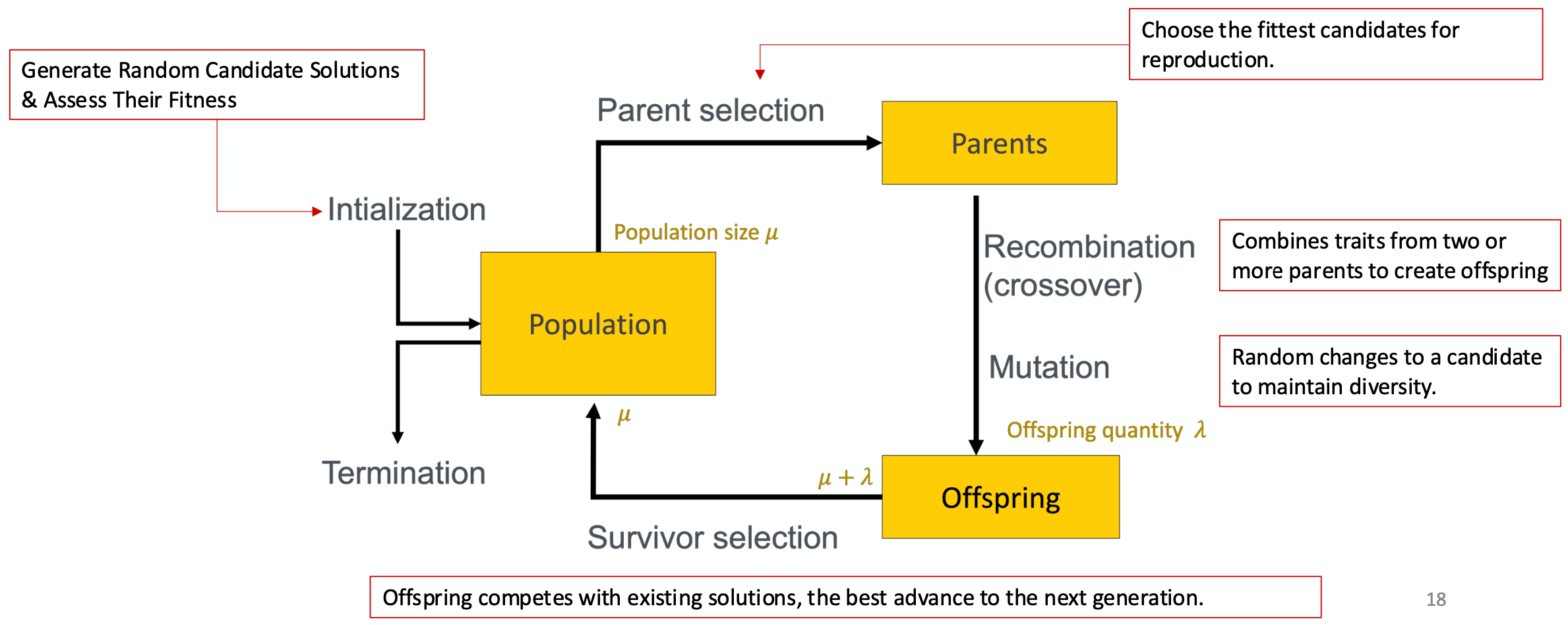
(image borrowed from my professor)
The population is initialized by selecting a random subset of the search space.
There are two inherent, competing forces in evolutionary algorithms. The process of recombination (reproduction) and mutation promotes diversity and represents a push towards novelty. The process of selecting the fittest parents or survivors decreases diversity and represents a push towards quality. By going back and forth between these two forces, evolutionary algorithms balance exploration and exploitation to find optimal results.
Balancing exploration and exploitation is crucial to avoid inefficiency or premature convergence. Premature convergence is the effect of losing population diversity too quickly and getting trapped in a local minimum.
Evolutionary Algorithm Components: Representation
Recall that earlier we were representing board configurations using coordinates and vectors (permutation encoding). In biological terms, what we were doing was mapping phenotypes (real-world solutions) to genotypes (encoded solutions).
A phenotype is the set of observable characteristics of an organism. A genotype is the complete set of genetic material of an organism.
Continuing with the biology theme, a solution is called a chromosome. A chromosome contains genes, which contain the values of the chromosome. The actual values are called alleles.
Loosely, genes are like the slots in a chromosome and the alleles are the values in those slots.
Evolutionary Algorithm Components: Evaluation (Fitness) Function
Once we have encoded representations of the inputs, we can programmatically assess their quality. This is where the objective function we saw earlier comes in.
In the phenotype space, the function is called an objective function. In the genotype space, the function is called a fitness function.
The fitness function assigns a numerical value (referred to as fitness value) to each phenotype so that the algorithm can know which ones to select for recombination. Typically, the "fittest" individuals have high fitness values, so we seek to maximize fitness.
Evolutionary Algorithm Components: Population
Formally, a population is a multiset of candidate solutions. This means that repeated elements are allowed to exist in the population.
A population is considered to be the basic unit of evolution. So a population evolves, not single individuals.
Diversity of a population can refer to either fitness diversity or phenotype/genotype diversity.
Evolutionary Algorithm Components: Selection Mechanism
The selection mechanism compares the fitness values of the solutions to decide which ones become parents.
Even though the general goal is to push the population towards higher fitness, the selection mechanism is usually probabilistic. Higher-quality solutions are more likely to be selected, but sub-optimal (or even the worst) solutions can still be picked.
Even though it might seem like it makes the most sense to just pick the solutions with the highest fitness values, it's sometimes necessary to not do that. Evolutionary algorithms can get stuck in a local maximum, and the only way to get out would be to pick sub-optimal solutions. Biologically, this is referred to as "genetic drift".
An example of a selection mechanism is a roulette wheel. Suppose we have three solutions `A, B, C`. `A` has a fitness of `3`; `B` has a fitness of `1`; `C` has a fitness of `2`. We can put them on a roulette wheel like so:
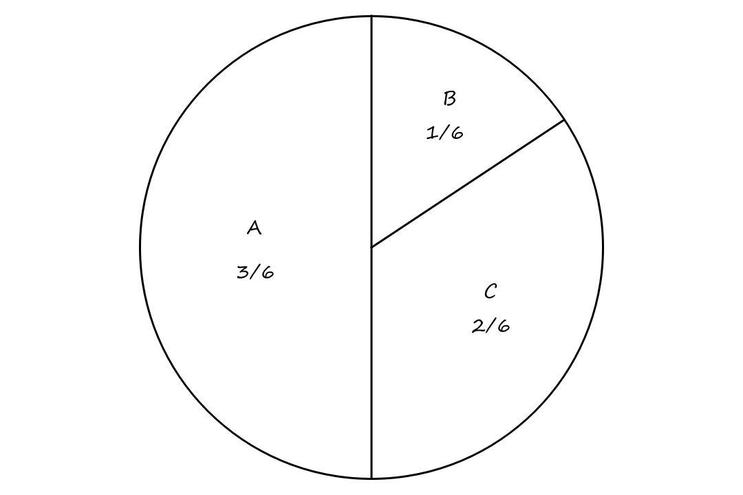
This way, `A`, which has the highest fitness value, has the highest chance of being selected.
The selection mechanism is also responsible for replacing the elements in the population with survivors.
While parent selection is usually probabilistic, survivor selection is usually deterministic. The process can be fitness based (compare the fitness values of the parents + offspring) or age based (replace as many parents as possible with offspring).
Evolutionary Algorithm Components: Recombination
Once the parents are selected, the offspring need to be produced. Recombination is the process of merging information from the parents into the offspring. The choice of what information to merge is random, so it's possible that the offspring can be worse or the same as the parents.
Evolutionary Algorithm Components: Termination
The algorithm has to stop eventually. There are several conditions we can use to determine when to stop:
- reaching some desired level of fitness
- reaching the maximum allowed number of generations
- reaching some level of diversity
- reaching some number of generations without fitness improvement
Variation Operators
Variation operators are genetic information manipulators that generate new candidate solutions. Mutation and recombination are the typical variation operators that are used in evolutionary algorithms. Variation operators are necessary for introducing diversity into the population.
Binary Representation
Suppose that we are encoding our solutions using strings of `1`s and `0`s (the genotype space is the set of strings of binary digits).
One problem we would do this for is the knapsack problem, in which we are deciding which items to put in a knapsack to maximize item value/count and minimize wasted bag space. A `1` would mean put the item in the knapsack and a `0` would mean don't.
Mutation
One simple mutation we can do is to randomly flip bits. For example, `10100 rarr 00010`.
Formally, each bit has a probability `p_m` of flipping. `p_m` is referred to as the mutation rate. It's typically between `1/text(population size)` and `1/text(solution length)`.
Using a lower probability preserves high-fitness individuals while using a higher probability encourages exploration (but risks disrupting good solutions). Generally, if we want to optimize overall population fitness, then we use a lower probability. If we want to find a single high-fitness individual, then using a higher probability can be better.
There's an interesting problem with using binary. Consider the numbers `6`, `7`, and `8`, which are `0110`, `0111`, and `1000` in binary respectively.
It takes only `1` bit flip to go from `0110` to `0111`, but it takes `4` bit flips to go from `0111` to `1000`. As a result, the probability of changing `7` to `8` is much less than the probability of changing `6` to `7`.
Gray coding, which is a variation on the binary representation such that consecutive numbers differ in only one bit, helps with this problem.
`1`-Point Crossover
One simple crossover technique we can do is to choose a random point and swap the parents' info at that point to produce the children.
| `0` | `0` | `0` | `0` | `0` | `0` | `0` |
| `1` | `1` | `1` | `1` | `1` | `1` | `1` |
Using the red line as the crossover point, we get
| `0` | `0` | `0` | `0` | `1` | `1` | `1` |
| `1` | `1` | `1` | `1` | `0` | `0` | `0` |
There is a positional bias when using a `1`-point crossover. Genes that are near each other are more likely to stay near each other and genes from opposite ends of the string can never be kept together.
`n`-Point Crossover
Instead of picking just `1` split point, we can pick `n` split points.
| `0` | `0` | `0` | `0` | `0` | `0` | `0` | `0` | `0` | `0` | `0` | `0` | `0` |
| `1` | `1` | `1` | `1` | `1` | `1` | `1` | `1` | `1` | `1` | `1` | `1` | `1` |
produces
| `0` | `0` | `0` | `0` | `1` | `1` | `1` | `0` | `0` | `0` | `0` | `0` | `1` |
| `1` | `1` | `1` | `1` | `0` | `0` | `0` | `1` | `1` | `1` | `1` | `1` | `0` |
Uniform Crossover
Another type of crossover we can do is to randomly pick genes from each parent. For the first child, each gene has a `50%` chance to come from one of the parents. Then the second child is created by flipping each gene of the first child.
| `0` | `1` | `0` | `0` | `1` | `0` | `1` | `1` | `0` | `0` | `0` | `1` | `0` | `1` | `1` | `0` | `0` | `1` |
| `1` | `0` | `1` | `1` | `0` | `1` | `0` | `0` | `1` | `1` | `1` | `0` | `1` | `0` | `0` | `1` | `1` | `0` |
Integer Representation
Now let's look at variation operators for solutions that are encoded using more numbers than just `1` and `0`.
An example of a problem where we would use this type of encoding is graph coloring, where the goal is to color each vertex so that no two vertices share the same color. We would use numbers to represent each color.
Mutation
For each gene, we could add a small (positive or negative) value with some probability `p`. We could also replace the gene with a random value with some probability `p`.
Recombination
The same recombination techniques we saw for the binary representation can be used for the integer representation as well.
Permutation Representation
Some problems, like the `n`-queens problem, require that solutions do not contain repeated values. For these types of problems, the order in which events occur matters a lot, like planning a route or scheduling jobs.
Swap Mutation
We can choose `2` alleles and swap them.
| `1` | `3` | `5` | `4` | `2` | `8` | `7` | `6` |
`darr`
| `1` | `3` | `7` | `4` | `2` | `8` | `5` | `6` |
Insert Mutation
We can choose `2` alleles and move the second one up to the first one.
| `1` | `2` | `3` | `4` | `5` | `6` | `7` | `8` |
`darr`
| `1` | `2` | `5` | `3` | `4` | `6` | `7` | `8` |
Scramble Mutation
We can pick a subset of genes and randomly rearrange the alleles in those positions.
| `1` | `2` | `3` | `4` | `5` | `6` | `7` | `8` |
`darr`
| `1` | `3` | `5` | `4` | `2` | `6` | `7` | `8` |
These types of mutations (swap, insert, scramble) are preferred for order-based problems, i.e., problems where the order of events are important.
Inversion Mutation
We can pick `2` alleles and invert the substring between them.
| `1` | `2` | `3` | `4` | `5` | `6` | `7` | `8` |
`darr`
| `1` | `5` | `4` | `3` | `2` | `6` | `7` | `8` |
This preserves most of the adjacency information (since it only breaks `2` links) but it is disruptive for the order information.
When performing mutations on permutations, we can't consider each gene independently since it might mess up the permutation. So the mutation parameter is the probability that a chromosome undergoes mutation, instead of the probability that each gene undergoes mutation, like in the binary and integer case.
Partially Mapped Crossover (PMX)
Doing a simple crossover for permutations isn't straightforward. It was implied in the `8`-queens problem, but doing a simple substring swap(s) will most likely not preserve the permutation property.
Suppose we have two parents
| `1` | `2` | `3` | `4` | `5` | `6` | `7` | `8` | `9` |
| `9` | `3` | `7` | `8` | `2` | `6` | `5` | `1` | `4` |
The first step of PMX is to choose `2` crossover points and copy the segment between them from the first parent into the first child.
| `1` | `2` | `3` | `4` | `5` | `6` | `7` | `8` | `9` |
| `9` | `3` | `7` | `8` | `2` | `6` | `5` | `1` | `4` |
First child:
| - | - | - | `4` | `5` | `6` | `7` | - | - |
The second step is to look at the segment in the second parent and see which values weren't copied over to the first child. In this example, `8` and `2`.
| `1` | `2` | `3` | `4` | `5` | `6` | `7` | `8` | `9` |
| `9` | `3` | `7` | `8` | `2` | `6` | `5` | `1` | `4` |
What we do with these uncopied values is best explained with a visual.
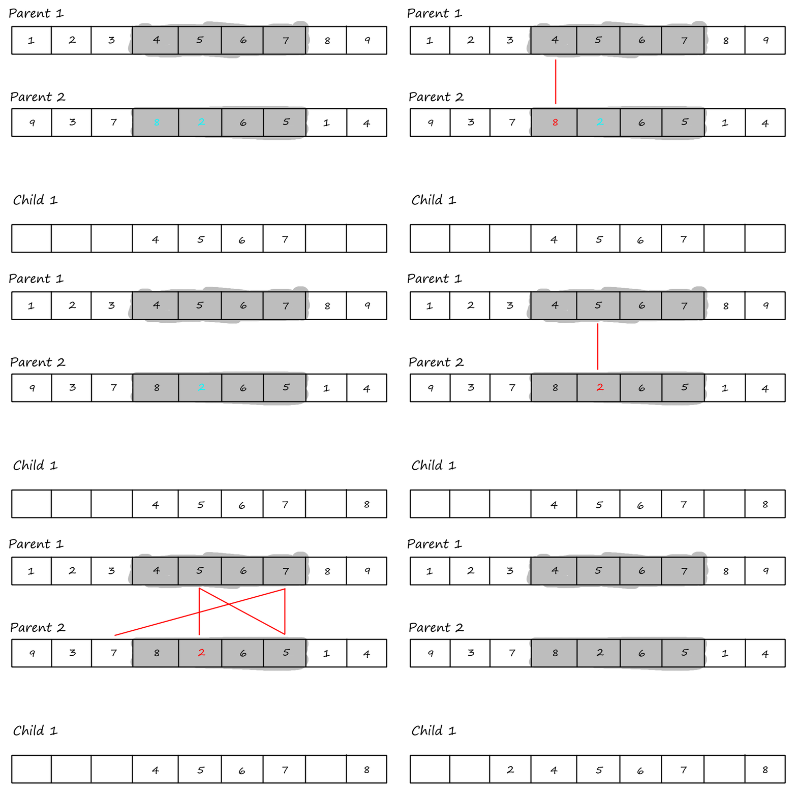
The last step is to copy the remaining values from the second parent into the same positions in the first child.
| `1` | `2` | `3` | `4` | `5` | `6` | `7` | `8` | `9` |
| `9` | `3` | `7` | `8` | `2` | `6` | `5` | `1` | `4` |
First child:
| `9` | `3` | `2` | `4` | `5` | `6` | `7` | `1` | `8` |
The second child is produced the same way, just with the parent roles reversed (so the second parent's segment is copied into the second child as the first step).
Order `1` Crossover
The first step of the order `1` crossover is the same as the first step of PMX: choose `2` crossover points and copy the segment between them from the first parent into the first child.
| `1` | `2` | `3` | `4` | `5` | `6` | `7` | `8` | `9` |
| `9` | `3` | `7` | `8` | `2` | `6` | `5` | `1` | `4` |
First child:
| - | - | - | `4` | `5` | `6` | `7` | - | - |
Then we copy the values from the second parent that weren't copied over yet, starting from the right of the rightmost crossover point and wrapping around to the beginning when we reach the end.
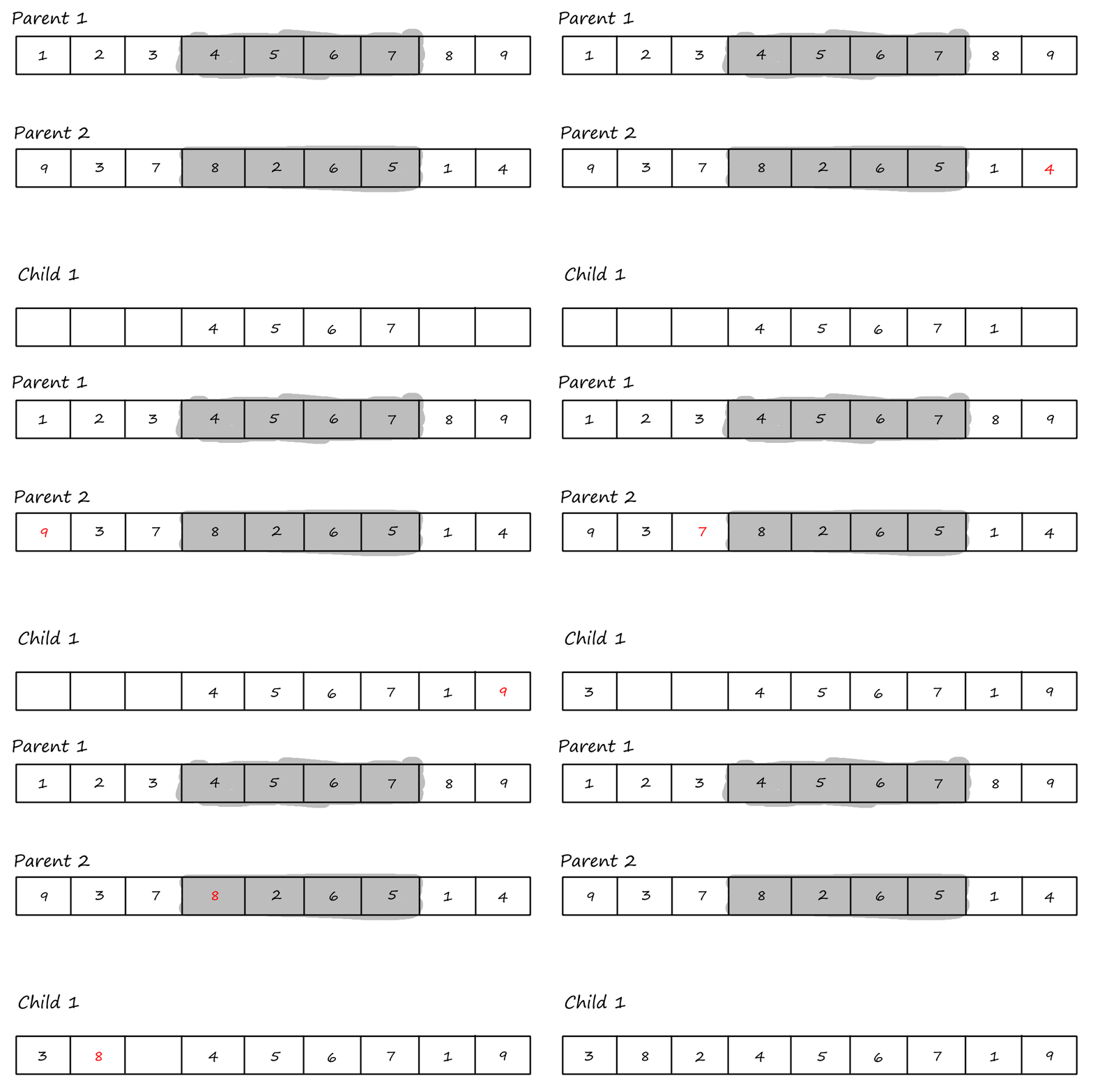
First child:
| `3` | `8` | `2` | `4` | `5` | `6` | `7` | `1` | `9` |
The second child is produced the same way, just with the parent roles reversed (so the second parent's segment is copied into the second child as the first step).
The goal of order crossover is to transmit information about relative order from the second parent.
Cycle Crossover
For this crossover technique, we copy cycles from the parents into the children. Cycles are found using the same visual method in PMX.
Cycle 1:
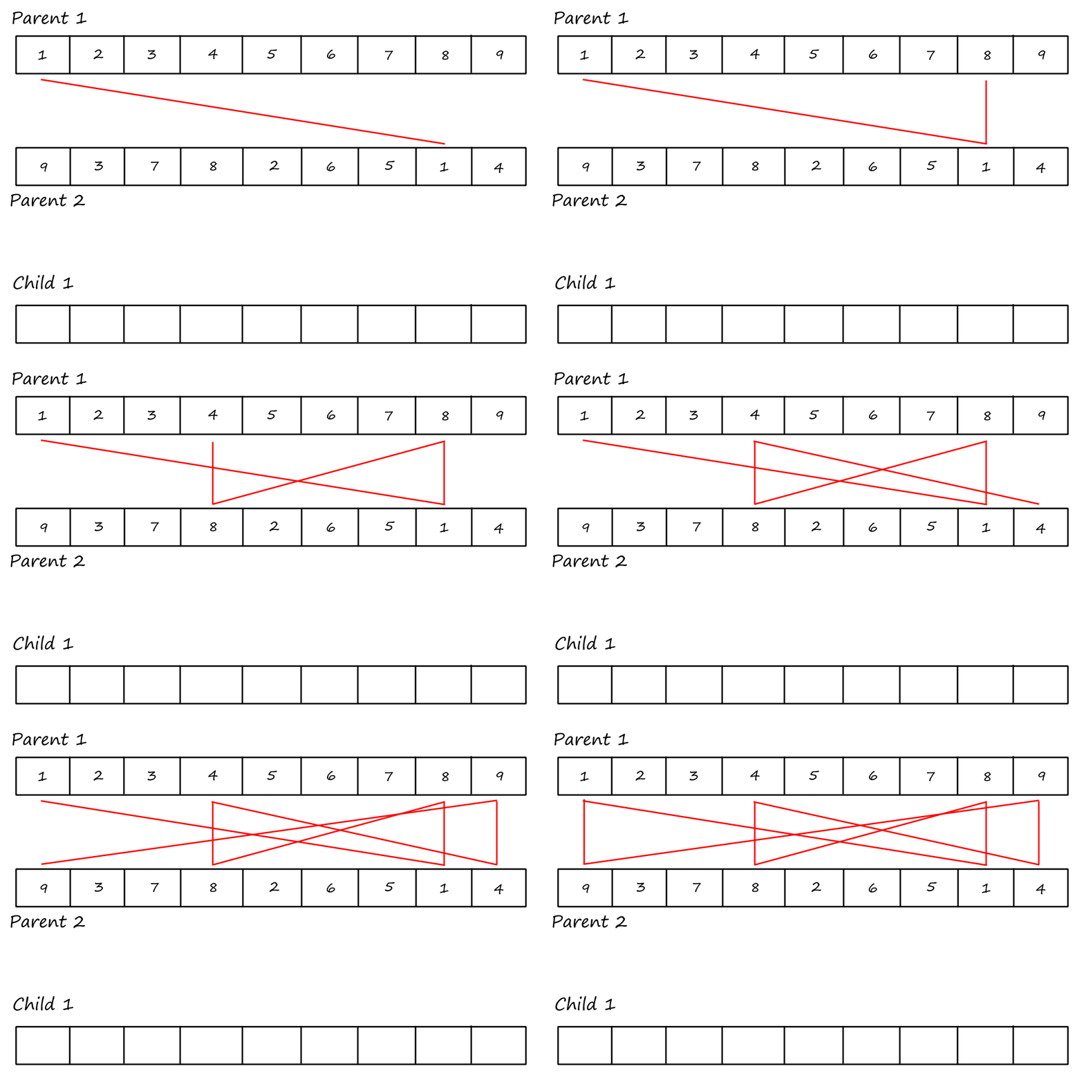
I (obviously) reused the same image and forgot to remove the "Child `1`".
Cycle 2:
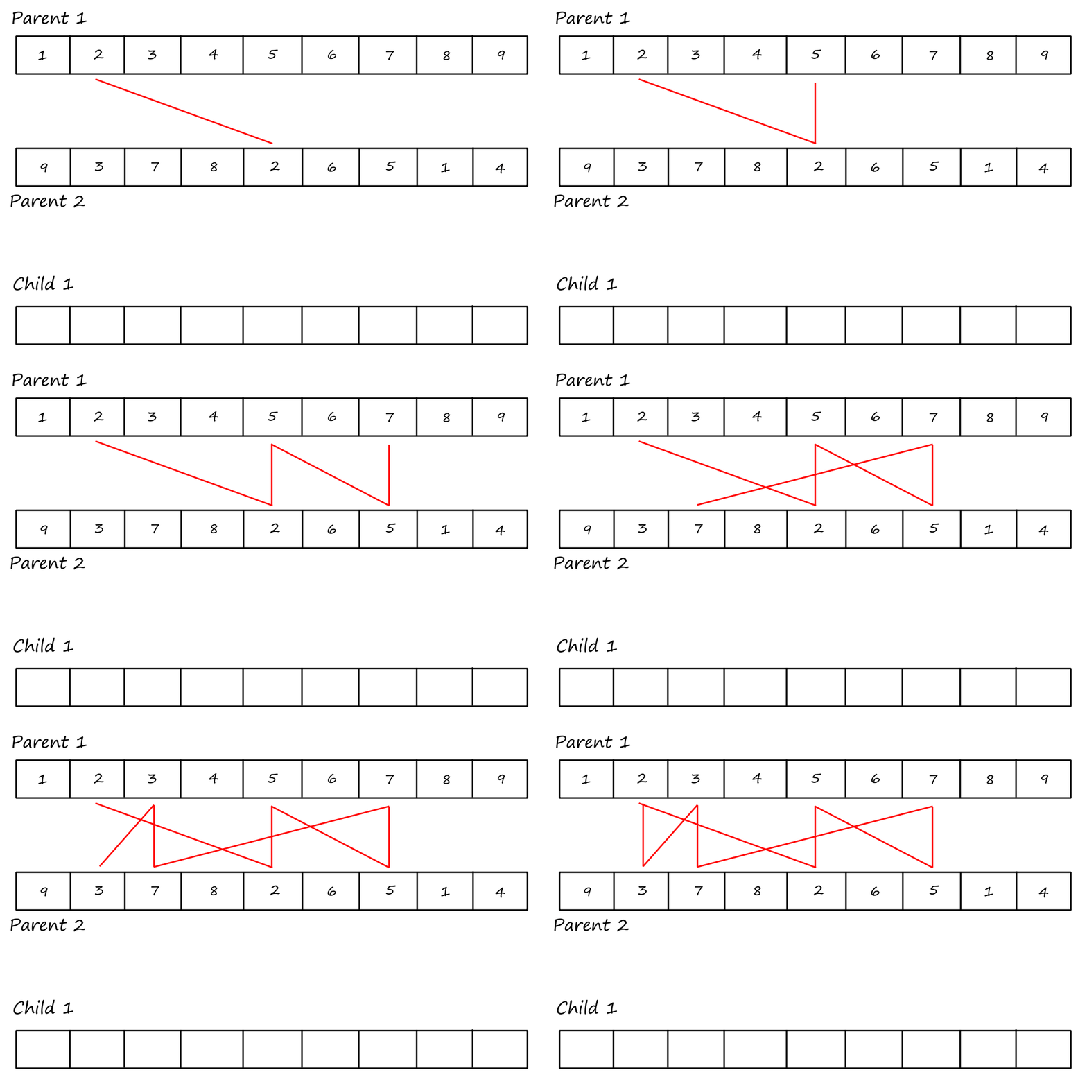
I (obviously) reused the same image and forgot to remove the "Child `1`".
So we take the values involved in the first cycle and copy them into the children in their respective positions.
First child:
| `1` | - | - | `4` | - | - | - | `8` | `9` |
Second child:
| `9` | - | - | `8` | - | - | - | `1` | `4` |
Then we take the values involved in the second cycle and copy them into the children, but in the opposite positions (so the values from the first parent go into the second child and the values from the second parent go into the first child).
First child:
| `1` | `3` | `7` | `4` | `2` | - | `5` | `8` | `9` |
Second child:
| `9` | `2` | `3` | `8` | `5` | - | `7` | `1` | `4` |
Then we take the values involved in the third cycle and copy them into the children in their respective positions.
First child:
| `1` | `3` | `7` | `4` | `2` | `6` | `5` | `8` | `9` |
Second child:
| `9` | `2` | `3` | `8` | `5` | `6` | `7` | `1` | `4` |
And we keep repeating this alternating pattern until we're done.
The goal of cycle crossover is to transmit information about the absolute position in which elements occur.
Real-Valued/Floating-Point Representation
A solution is represented as a vector `[x_1, x_2, ..., x_k]^T` where each `x_i in RR`.
Uniform Mutation
We could replace each element with a randomly-selected value from some predefined range of values. (This is similar to bit flipping in the binary representation and random resetting in the integer representation.)
Uniform mutation is most suitable when the genes encode cardinal attributes, since all values are equally likely to be chosen.
Nonuniform Mutation
The most common method is to add a random delta to each gene, where the delta is taken from a Gaussian distribution with mean `0` and standard deviation `sigma`.
`x_i' = x_i + N(0, sigma)`
`sigma` is the standard deviation (also referred to here as the mutation step size) and it controls how big the deltas are.
Discrete Crossover
A simple crossover technique is to take an allele from one of the parents with equal probability.
Intermediate Crossover (Arithmetic Recombination)
Since we're dealing with real numbers, we can create children that are "between" the parents. For two parents `x,y`, we can create a child `z` using
`z_i = alpha x_i + (1-alpha) y_i`
for `0 le alpha le 1`
where `alpha` can be constant, variable, or picked randomly every time.
Single Arithmetic Crossover
We can do this for only one gene:
`[x_1, ..., x_(k-1), alpha*y_k+(1-alpha)*x_k,...,x_n]`
(exact copy of parent `x` except for the `k^(th)` gene)
Simple Arithmetic Crossover
For several genes:
`[x_1, ..., x_k, alpha*y_(k+1)+(1-alpha)*x_(k+1),...,alpha*y_n+(1-alpha)*x_n]`
(exact copy of parent `x` except for genes `k+1` to `n`)
Whole Arithmetic Crossover
Or for all the genes:
`z=alpha*x+(1-alpha)*y`
Crossover vs. Mutation
Crossover is explorative and mutation is exploitative.
Only crossovers can combine information from two parents.
Only mutation can introduce new information.
Hitting the optimum usually requires a lucky mutation.
Selection Operators
Selection operators are used for population management. They decide which individuals in the population are selected for mating (parent selection) and which individuals in the population survive (survivor selection).
Selection pressure is the intensity with which fitter individuals are favored over worse individuals. A higher selection pressure means that fitter individuals are more favored, and a lower selection pressure means that worse individuals have a higher chance of being selected.
Parent Selection
Fitness Proportional Selection
For parent selection, it's natural to want to use higher-fitness individuals for mating. But, as mentioned before, using only high-fitness individuals can have problems with getting stuck at local optima.
Fitness proportional selection is a probabilistic method that selects individuals for mating by their absolute fitness values. Individuals with a higher fitness have a higher chance of being selected. And since we're looking at absolute fitness values, individuals with much higher fitness have a much higher chance of being selected.
`P_(FPS)(i)=f_i/(sum_(j=1)^(mu)f_j)`
For example, suppose we have some individuals `x=1, x=2, x=3` with their fitness values given below.
| `x` | fitness |
|---|---|
| `1` | `1` |
| `2` | `4` |
| `3` | `9` |
We could simulate fitness proportional selection by making copies of each individual based on their fitness values. This way, if we select one copy, the probability that the copy is going to have a high fitness value is high. Individual `x=3` has a `9/14` chance of being selected versus individual `x=1`, which only has a `1/14` chance of being selected.
| `1` | `2` | `2` | `2` | `2` | `3` | `3` | `3` | `3` | `3` | `3` | `3` | `3` | `3` |
One of the disadvantages of using fitness proportional selection is that it could lead to premature convergence. Since higher-fitness individuals have a significantly higher chance of being selected, the population could quickly lose diversity and converge to a single solution.
Another disadvantage of fitness proportional selection is that it is highly susceptible to function transposition. Consider the following fitness values and selection probabilities.
| Individual | Fitness for `f` | Selection probability for `f` | Fitness for `f+10` | Selection probability for `f+10` | Fitness for `f+100` | Selection probability for `f+100` |
|---|---|---|---|---|---|---|
| `A` | `1` | `0.1` | `11` | `0.275` | `101` | `0.326` |
| `B` | `4` | `0.4` | `14` | `0.35` | `104` | `0.335` |
| `C` | `5` | `0.5` | `15` | `0.375` | `105` | `0.339` |
| Sum | `10` | `1.0` | `40` | `1.0` | `310` | `1.0` |
We can see the selection probabilities don't stay proportional to the fitness values as we change the fitness values. `C` is `4` points higher than `A`, and in the simple case of `f`, has a much higher chance of being selected. In the case of `f+100`, `C` is still `4` points higher than `A`, but `C` has virtually the same chance of being selected as `A`.
Windowing
One way of dealing with this is to use windowing. Windowing is a method that adjusts the fitness values dynamically to maintain the fitness differentials.
Let `beta^t` be the worst fitness in the `t^(th)` generation. We adjust the fitness values every generation by using
`f'(i)=f(i)-beta^t`
This essentially makes it so that the worst individual has a zero chance of being picked while still allowing high-fitness invidivudals to maintain their high probability.
Sigma Scaling
Sigma scaling adjusts the fitness values by incorporating the population variance. Let `bar f` be the mean of the fitness values, `sigma_f` be the standard deviation, and `c` be some constant value (usually `2`). We adjust the fitness values every generation by using
`f'(i)=max(0, f(i)-(bar f - c*sigma_f))`
Rank-based Selection
Of course, we could avoid the problems of fitness proportional selection by using something else entirely. Instead of looking at absolute fitness, we could look at relative fitness.
For example, in the earlier example, `x=1` had a `1/14` chance of being selected and `x=3` had a `9/14` chance of being selected. Looking at absolute fitness, `x=3` is `9` times more likely to be selected than `x=1`.
If we want to look at relative fitness, let's assign some rank to these individuals, say rank `2` to `x=3`, rank `1` to `x=2`, and rank `0` to `x=1` (so the higher the rank, the higher the fitness). Assigning a rank allows us to know which individual is the fittest without being biased by how much fitter an individual is.
| `x` | fitness | rank |
|---|---|---|
| `1` | `1` | `0` |
| `2` | `4` | `1` |
| `3` | `9` | `2` |
Ranking introduces a sorting overhead, but this is usually negligible compared to the overhead of computing fitness values.
Linear Ranking
`P(i)=(2-s)/mu+(2i(s-1))/(mu(mu-1))`
`s` is the selection pressure, and it ranges from `1 lt s le 2`. Using a higher selection pressure favors fitter individuals.
| Individual | Fitness | Rank | `P_(FPS)` | `P_(LR)` for `s=2` | `P_(LR)` for `s=1.5` |
|---|---|---|---|---|---|
| `A` | `1` | `0` | `0.1` | `0` | `0.167` |
| `B` | `4` | `1` | `0.4` | `0.33` | `0.33` |
| `C` | `5` | `2` | `0.5` | `0.67` | `0.5` |
| Sum | `10` | - | `1.0` | `1.0` | `1.0` |
One limitation with linear ranking is that the selection pressure is limited. It can only take on values between `1` and `2`*. So the fittest individual only has at most a `2` times higher chance of being selected.
*Having `s gt 2` would lead to negative probabilities for less fit individuals since all the probabilities have to add up to `1`.
Exponential Ranking
`P(i)=(1-e^(-i))/c`
where `c` is a normalization constant that ensures the sum of all the probabilities add up to `1`.
Exponential ranking is preferred over linear ranking when we want the fittest individuals to have more chances of being selected. This is helpful in situations where it is really costly to compute fitness values, so we only want to spend resources calculating fitness values for individuals that are worth calculating.
Tournament Selection
If the population is very large, then it can be very expensive to keep computing the fitness of the whole population. Instead, we can pick `k` members at random and then select the best individuals from that sample.
The probability of selecting an individual `i` is based on several factors:
- the rank of `i`
- `k`, the size of the sample
- a higher `k` increases selection pressure
- whether individuals are picked with replacement
- picking without replacement increases selection pressure
- whether the fittest individual always wins (deterministic) or whether they win probabilistically
Population Management
When the selected parents produce offspring, they have to replace individuals in the population to maintain the population size.
We'll use `mu` for the population size and `lambda` for the number of offspring.
Generational Model
In the generational model, the whole population is replaced (assuming two parents produce two children). This results in a faster exploration of the search space. But it is also more likely to remove good traits from the population that are beneficial for producing good solutions.
For each generation, `lambda=mu`.
Steady-State Model
In the steady-state model, only some of the population is replaced. The proportion of the population that is replaced is called the generational gap (represented by `lambda/mu`).
For each generation, `lambda lt mu`.
Survivor Selection
The selection methods for selecting individuals to be replaced can be age-based or fitness-based. Age-based methods are not interesting, so we'll only look at fitness-based ones.
Elitism
As the name suggests, the fittest individuals remain in the population while less fit individuals are replaced. This ensures that there is always at least one copy of the fittest solution in the population.
GENITOR (Delete Worst)
As the name suggests, the worst members of the population are selected for replacement. To be honest, I still don't understand the difference between elitism and GENITOR.
Round-Robin Tournament
Here, the offspring is merged with the population and they duke it out with each other to see who wins. Each individual is evaluated against `q` other randomly chosen individuals. The individuals with the most wins stay in the population.
When `q` is large, the selection pressure is higher since stronger individuals are more likely to survive. `q` is typically `10`.
`(mu,lambda)`-Selection
From what I understand, `mu` parents generate `lambda` offspring, and only the best `mu` children are selected to replace the whole population. (This requires `lambda gt mu`.)
`(mu+lambda)`-Selection
Here, the offspring is merged with the population and the best `mu` individuals survive.
Selection Pressure
As mentioned earlier, the idea behind selection pressure is that fitter individuals are more likely to survive or be chosen as parents.
Selection pressure can be quantified by a measure called takeover time (denoted as `tau^(ast)`). Takeover time is the number of generations it takes for the fittest individual to take over the entire population.
The general formula for takeover time is
`tau^(ast)=ln(lambda)/ln(lambda/mu)`
For example, for `mu=15` and `lambda=100`, `tau^(ast)~~2`, which means that in `2` generations, every individual will be the same (the best individual).
For fitness proportional selection, the takeover time is
`tau^(ast)=lambda ln(lambda)`
Evolutionary Algorithm Variants
As we've seen, there are many choices for which representation, selection operators, and variation operators to use. The set of choices that are used defines an "instance" of an evolutionary algorithm.
Historically, many different types of evolutionary algorithms have been developed.
Genetic Algorithms
The genetic algorithm (GA) was developed in the 1960s by Holland in his study of adaptive behavior.
| Representation | Bit-strings |
| Recombination | 1-Point crossover |
| Mutation | Bit flip |
| Parent selection | Fitness proportional - implemented by Roulette Wheel |
| Survivor selection | Generational |
The mutation probability is typically low since there is more emphasis on recombination as the preferred way of generating offspring.
GA is typically used for straightforward binary representation problems, function optimization, and teaching evolutionary algorithms.
Evolution Strategies
Evolution strategies (ES) were developed in the 1960s by Rechenberg and Schwefel in their study of shape optimization.
| Representation | Real-valued vectors |
| Recombination | Discrete or intermediary |
| Mutation | Gaussian perturbation |
| Parent selection | Uniform random |
| Survivor selection | Deterministic elitist replacement by `(mu, lambda)` or `(mu+lambda)` |
| Specialty | Self-adaptation of mutation step sizes |
Self-adaptation means that the mutation step size changes from generation to generation. This is implemented by Rechenberg's `1//5` success rule, which scales `sigma` by a factor depending on the success rate of a mutation (whatever that means).
Here are some different types of recombination methods. `i` is the index of the gene, `x` and `y` are the parents, and `z` is the child.
| Two fixed parents | Two parents selected for each `i` | |
|---|---|---|
| `z_i=(x_i+y_i)/2` | local intermediary | global intermediary |
| `z_i` is `x_i` or `y_i` chosen randomly | local discrete | global discrete |
ESs typically use global recombination.
`(mu,lambda)` selection is generally preferred over `(mu+lambda)` selection because `(mu+lambda)` has a tendency to keep bad solutions (and the traits that produce the bad solutions) around for a large number of generations.
ESs are typically used for numerical optimization and shape optimization.
Evolutionary Programming
Evolutionary programming (EP) was developed in the 1960s by Fogel et al. in their study of generating artificial intelligence (by attempting to simulate evolution as a learning process).
| Representation | Real-valued vectors |
| Recombination | None |
| Mutation | Gaussian perturbation |
| Parent selection | Deterministic (each parent creates one offspring via mutation) |
| Survivor selection | Probabilistic `(mu+mu)` |
| Specialty | Self-adaptation of mutation step sizes |
The notable thing about EP is that there is no recombination. This is because each individual is seen as a distinct species, so it doesn't make sense theoretically to perform recombination. This also means that only `1` parent is needed to produce a child, so there's not really a parent selection mechanism.
This has, of course, led to much debate and study on the performance of algorithms with and without recombination.
Survivor selection is implemented using stochastic round-robin tournaments.
EP is typically used for numerical optimization.
Genetic Programming
Genetic programming (GP) was developed in the 1990s by Koza.
| Representation | Tree structures |
| Recombination | Exchange of subtrees |
| Mutation | Random change in trees |
| Parent selection | Fitness proportional |
| Survivor selection | Generational replacement |
Similarly to GA, the mutation probability is low for GP. In fact, Koza suggested using a mutation rate of `0%`. The idea behind not needing mutation is that recombination already has a large shuffling effect, so it's kind of a mutation operator already.
For large population sizes, over-selection is a method that is used for parent selection.
The population is ranked by fitness, then split into two groups. One group contains the top `x%` and the other contains the remaining `(100-x)%`. `80%` of the selection operations come from the first group, and the other `20%` come from the other group.
GP is typically used for machine learning tasks, like prediction and classification.
Differential Evolution
Differential evolution (DE) was developed in 1995 by Storn and Price.
| Representation | Real-valued vectors |
| Recombination | Uniform crossover (with crossover probability `C_r`) |
| Mutation | Differential mutation |
| Parent selection | Uniform random selection of the `3` necessary vectors |
| Survivor selection | Deterministic elitist replacement (parent vs. child) |
The notable thing about DE is that `3` parents are needed to create a new child. We can see why when we look at how differential mutation works. Basically, the vector difference of two parents is added to another parent to produce the child.
Let `x,y,z` be the parents. The scaled vector difference of `y` and `z` is denoted as `p`, the perturbation vector. The child produced is denoted `x'`. `F` is the scaling factor that controls the rate at which the population evolves.
`p = F*(y-z)`
`x' = x + p`
For recombination, uniform crossover is used, meaning that each gene either comes from the first parent or the second parent. But there is a slight difference from the usual uniform crossover; there is a crossover probability `C_r in [0,1]` that decides the probability of picking the gene from the first parent.
DE is typically applied to nonlinear and nondifferentiable continuous space functions.
Parameters and Parameter Tuning
Each evolutionary algorithm variant differs in their choices for which operators to use. These choices are the parameters of the algorithm. There are two categories of parameters: symbolic parameters and numeric parameters.
Symbolic parameters are the categorical aspects of the algorithm. For example, what type of parent selection should be used? Or what type of recombination should be used?
Numeric parameters are the, well, numeric aspects of the algorithm. For example, what should the population size be? Or what should be the mutation probability?
Here's an example with three evolutionary algorithm instances `A_1`, `A_2`, and `A_3`.
| `A_1` | `A_2` | `A_3` | |
|---|---|---|---|
| symbolic parameters | |||
| representation | bitstring | bitstring | real-valued |
| recombination | `1`-point | `1`-point | averaging |
| mutation | bit-flip | bit-flip | Gaussian `N(0,sigma)` |
| parent selection | tournament | tournament | uniform random |
| survivor selection | generational | generational | `(mu,lambda)` |
| numeric parameters | |||
| `p_m` | `0.01` | `0.1` | `0.05` |
| `sigma` | n.a. | n.a. | `0.1` |
| `p_c` | `0.5` | `0.7` | `0.7` |
| `mu` | `100` | `100` | `10` |
| `lambda` | equal `mu` | equal `mu` | `70` |
| `k` | `2` | `4` | n.a. |
More formally, an evolutionary algorithm instance is a set of symbolic and numeric parameters.
`A_i=(S,N)`
`S={text(representation), text(recombination), text(mutation), text(parent selection), text(survivor selection)}`
`N={p_m, sigma, p_c, mu, lambda, k}`
where
- `p_m in [0,1]`
- `sigma in RR^+`
- `p_c in [0,1]`
- `mu in NN`
- `lambda in NN`
- `k in NN`
For two instances `A_i=(S_i,N_i)` and `A_j=(S_j,N_j)`, they are considered distinct evolutionary algorithms if at least one of the symbolic parameters is different.
`A_i ne A_j` if `S_i ne S_j`
They are considered variants of each other if they have the same symbolic parameters but different numeric parameters.
`A_i ~ A_j` if `S_i = S_j` and `N_i ne N_j`
In the above example, `A_1` and `A_2` are variants of each other and `A_1` and `A_3` are distinct algorithms.
Designing Evolutionary Algorithms
Abstractly, there are three layers for an evolutionary algorithm: the design layer, the algorithm layer, and the application layer. The design layer involves choosing the parameters to create the algorithm instance. I think the algorithm layer involves defining what type of evolutionary algorithm it is, like identifying it as a genetic algorithm for example. The application layer involves running the algorithm on a real-world problem.
With this, there are essentially two problems to solve: finding a solution to a real-world problem (optimization problem) and finding a set of parameters to design an algorithm to find those solutions (design problem). As a result, there are two types of quality assessments: one at the algorithm layer and one at the application layer.
At the algorithm layer, we have utility and testing. Utility is the measure of an EA's performance (e.g., number of fitness evaluations, algorithm runtime). Testing is the process of calculating and comparing utilities.
At the application layer, we have fitness and evaluation. Fitness is the measure of a solution's quality. Evaluation is the process of calculating and comparing fitness values.
The Tuning Problem
Parameter tuning refers to deciding what the parameters are before the algorithm is run.
Parameter control refers to adjusting the parameters while the algorithm is running. It can be deterministic (e.g., depending on how much time has passed), adaptive (changing based on the feedback from the search results), or self-adaptive (changing based on the quality of the solutions).
A tuner is a search algorithm that looks for the best set of parameters. In order to test a tuner's performance, we need a utility function that assigns a performance score to the tuner. Some measures that could be used for utility are mean best fitness and average number of evaluations to a solution.
Tuning by Generate-and-Test
The general flow for tuning is to generate sets of parameters and test each set. Since EAs are stochastic, the testing needs to be repeated several times. (Depending on the type of tuner -- iterative or non-iterative -- the generation of the parameters can happen once.)
Utility is defined formally as
`U(A_i)=bbb E(M(A_i,P))`
where
- `A_i` is the EA instance
- `P` is the problem instance
- `M(A_i,P))` is the performance metric (e.g., best fitness achieved, convergence speed)
- `bbb E` is the expected value
Utility is estimated by the testing process.
`hat U(A_i)=1/n sum_(j=1)^n M(A_i^((j)),P)`
where `n` is the number of runs and `A_i^((j))` is the algorithm used on the `j^(th)` run.
Multiobjective Evolutionary Algorithms
So far, we've been dealing with problems where the goal is to optimize only one objective function. But in the real world, most problems have multiple objectives that need to be minimized or maximized. For example, when buying a car, we want to find a nice balance between price and reliability.
Formally, the general multiobjective optimization problem (MOP) is defined as finding the decision variable vector
`bb x = [x_1, x_2, ..., x_n]^T`
that satisfies a set of constraints and optimizes a set of objective functions
`bb f(bb x) = [f_1(bb x), f_2(bb x), ..., f_k(bb x)]^T`
Dominance
Suppose we have two objective functions `f_1` and `f_2`, and we want to minimize both of them. `a,b,c,d,e` are solutions.
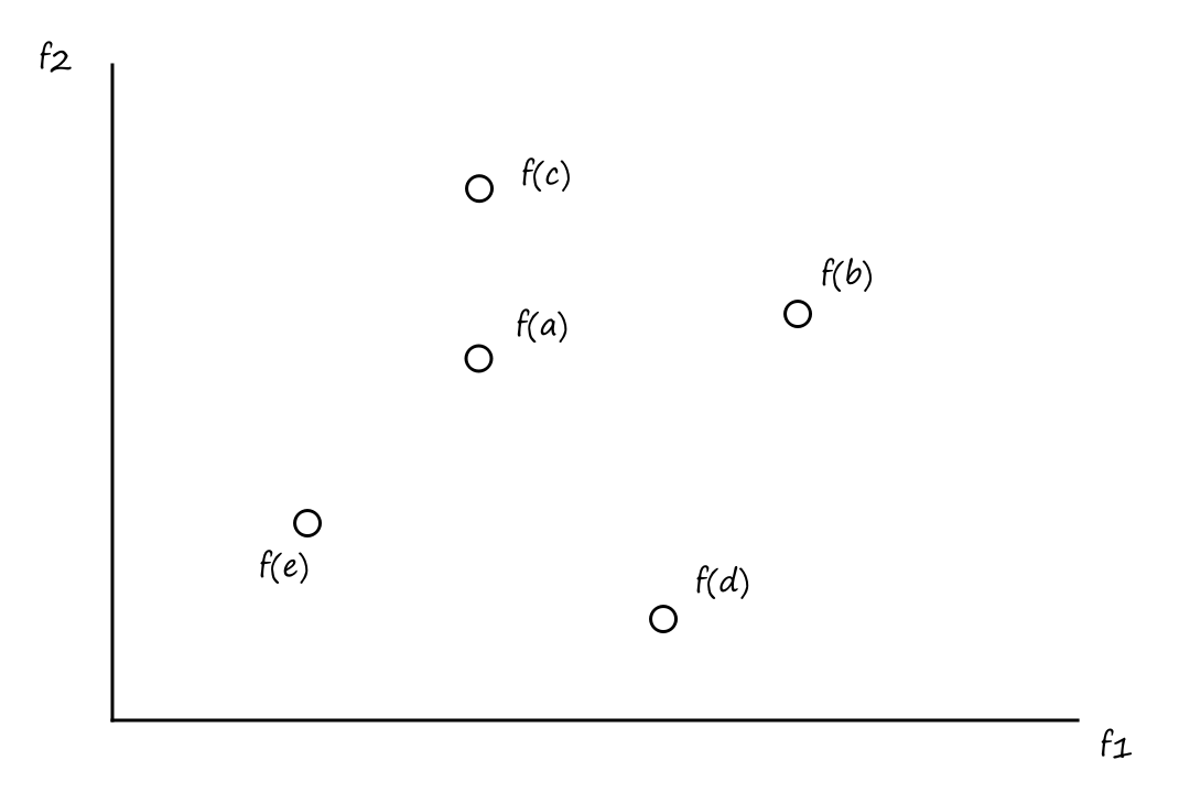
From this we can see that
- `a` is a better solution than `b` and `c`
- `a` is a worse solution than `e`
- `a` and `d` are incomparable
- `a` is better than `d` in terms of `f_1`, but `d` is better than `a` in terms of `f_2`
This introduces the concept of dominance. We say that `a` dominates `b` and `c`, and `e` dominates `a`.
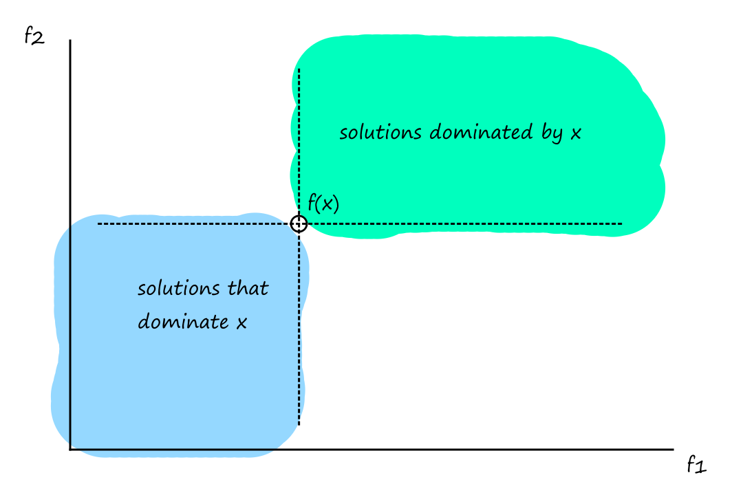
Formally, a solution `x` dominates a solution `y` if
- `x` is better than `y` in at least one objective
- `x` is not worse than `y` in all other objectives
`x` dominates `y` is written as
`x preceq y` for minimization
`x succeq y` for maximization
This is generally what it looks like for the minimization case:
Pareto Optimality
It's rare (at least I imagine it is) for there to exist one solution that optimizes all objective functions. More likely, there will be a set of solutions that are all fairly good, but they each have their own benefits and tradeoffs. These are referred to as Pareto optimal solutions.
In the example below, the green solutions are the Pareto optimal solutions. They're better than all the other solutions, but each Pareto optimal solution is not definitively better than any other Pareto optimal solution.
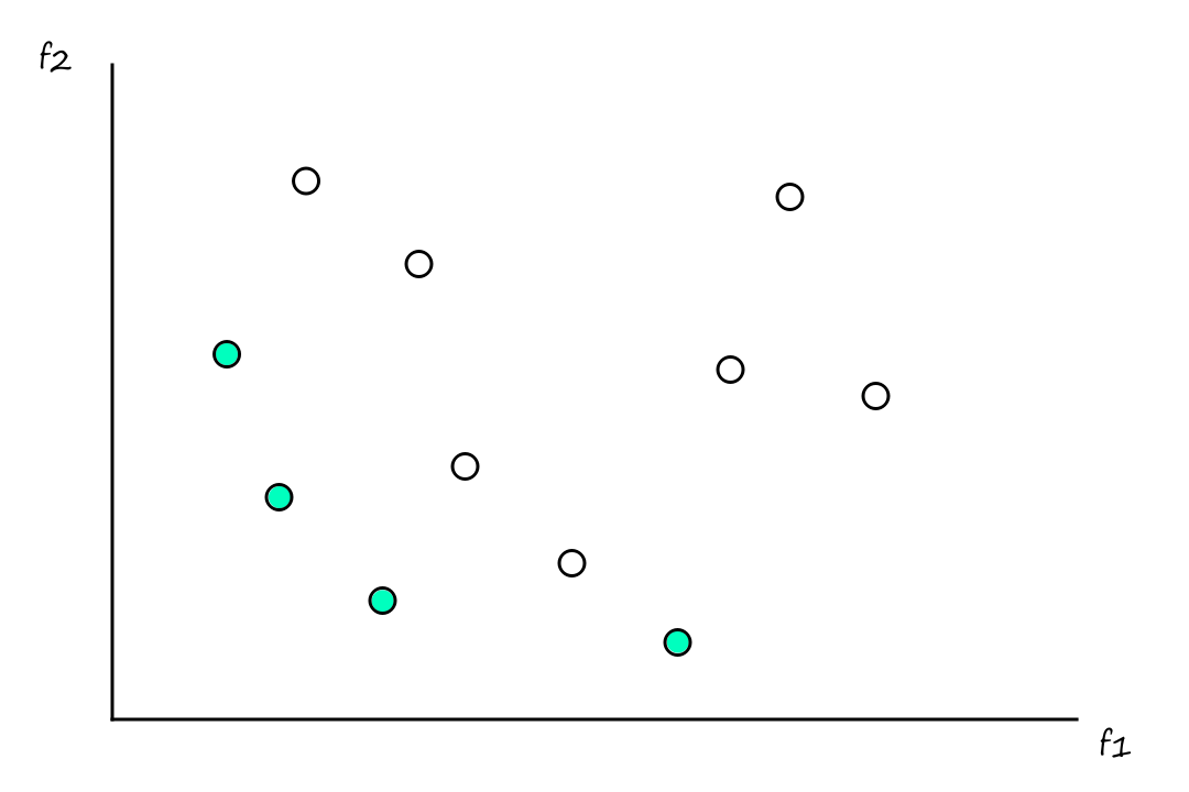
Formally, a solution `x` is non-dominated if no solution dominates `x`. A set of non-dominated solutions is the Pareto optimal set. The image (in the context of functions) of the Pareto optimal set is the Pareto optimal front.
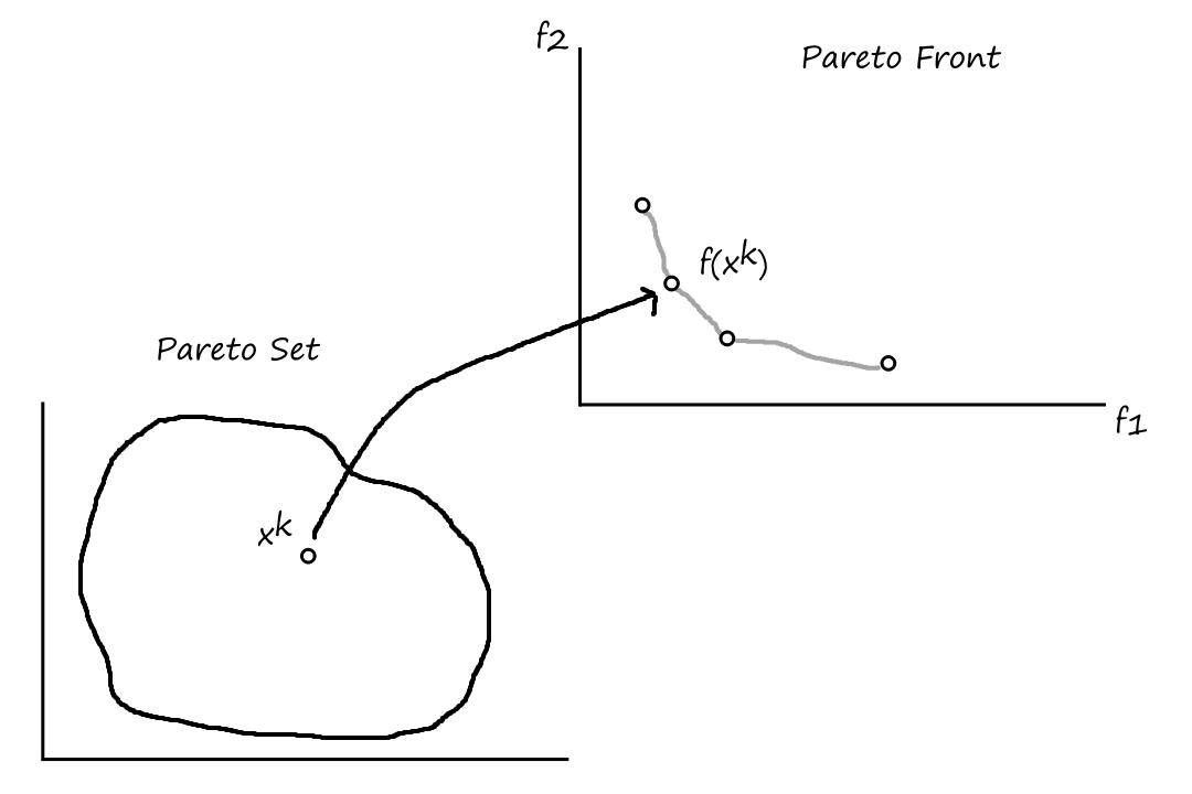
The set of Pareto optimal solutions is defined as
`cc P^(ast) = {x in Omega | not EE x' in Omega text( ) f(x') preceq f(x)}`
(there does not exist a solution that dominates a Pareto optimal solution)
The Pareto front is defined as
`cc P cc F^(ast) = {(f_1(x), ..., f_k(x)) | x in cc P^(ast)}`
Solving Multiobjective Problems
NSGA II
NSGA stands for Nondominated Sorting Genetic Algorithm. It is an algorithm that can find multiple Pareto optimal solutions in a single simulation run. It works by classifying individuals into layers based on dominance. For individuals that are in the same layer, the solution that is in the lesser crowded region is considered better.
MOEA/D
MOEA/D stands for Multiobjective Evolutionary Algorithm Based on Decomposition. It decomposes the optimization problem into `n` scalar optimization subproblems, which are solved in parallel.
LLMs
Generative AI is a type of AI that creates new content based on what it has learned from existing content. One example of a generative model is a large language model (LLM). At its core, LLMs are word predictors, that is, they generate text by predicting what words should be used.
For example, suppose we have the sentence, "When I hear rain on my roof, I _ in my kitchen." Using the surrounding words for context, an LLM makes predictions for what word(s) should go in the blank by assigning probabilties to word(s) that the LLM has seen in similar contexts. Some choices could be
- cook soup (`9.4%`)
- warm up a kettle (`5.2%`)
- nap (`3.6%`)
- relax (`2.5%`)
So how does predicting text relate to generating text? LLMs generate text by repeatedly predicting what word it thinks should come next after its own prediction.
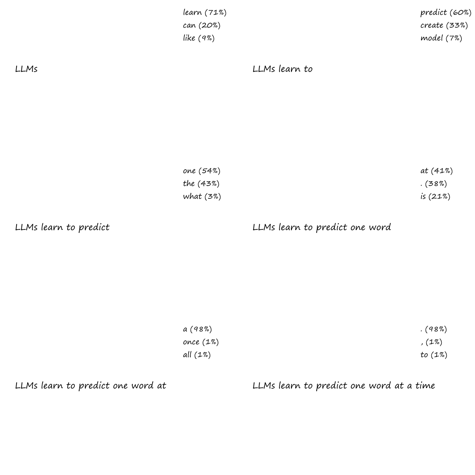
This is similar to how training is done for the LLM. The current group of words is the input and the target is the next word that comes next.

The first step in creating an LLM is to pretrain it on a large amount of text data. It's like literally feeding it a bunch of words so that it can develop a vocabulary.
The second step is to train it on a large amount of text data, except this time, the data is labeled. For example, we could give the LLM a bunch of sentences related to finance so that it learns what types of words are associated with finance. This type of training is called classification fine-tuning. There is another type of training called instruction fine-tuning where we give the LLM instructions (prompts) and sample answers so that it learns how certain questions/commands should be responded to.
After the first pretraining step, we end up with a foundation model that already has some basic capabilities, like text completion and typo recognition/correction. The second step is how we get more advanced LLMs.
Embeddings
LLMs don't actually understand words and text. They're like computers; they work with numbers. Words are converted into numbers, which the LLM performs calculations on to produce more numbers, which are converted back into words. The process of converting words into numbers is called embedding.
The basic idea behind embeddings is that words are assigned numerical values based on certain qualities or meanings of the word. So similar words, like words about finance, have similar numerical values.
More specifically, words are converted into continuous-valued vectors.
This `rarr [[-2.7], [-2.3], [8.9]]`
is `rarr [[-4.7], [-0.5], [6.2]]`
an `rarr [[6.2], [5.0], [-4.2]]`
example `rarr [[-0.1], [4.3], [-6.2]]`
Tokenizing
In order to create word embeddings, the text has to be split into individual tokens. A token can be thought of as an individual word.
For example, the sentence, "This is an example." can be tokenized into four tokens:
["This", "is", "an", "example."]
So a simple strategy for tokenizing a sentence is to split the sentence on spaces.
If we wanted to remove or tokenize punctuation, we could use regular expressions.
Once we have our tokens, we convert each token into a token ID. A simple way of doing this is to do
This `rarr 0`
is `rarr 1`
an `rarr 2`
example `rarr 3`
Let's say we wanted to build an LLM that can recognize phrases from books. To train it, we would give it a bunch of books to read. Programmatically, I suppose we would probably combine all the books into one large text file and feed that to the LLM. In order to know which text belongs to which book, we would need some sort of marker to indicate where one book ends and the next book begins. During the tokenization process, we use a special context token (e.g., <|endoftext|>) to handle this situation. Special context tokens also get converted into token IDs.
Another type of special context token is <|unk|> for handling unknown words (unknown to the LLM)
Now, (Back) to Embeddings
For simplicity, I'll continue with the assumption that a token is a word. So I'll use "token" and "word" interchangeably.
Each word in the LLM's vocabulary is initially assigned a vector of random values. These vectors form what is called the embedding matrix. A word's embedding vector is obtained by using the token ID to "index" into the embedding matrix.
`[[text(This)], [text(is)], [text(an)], [text(example)]] rarr [[-2.7, -2.3, 8.9], [-4.7, -0.5, 6.2], [6.2, 5.0, -4.2], [-0.1, 4.3, -6.2]]`
These random values get updated during the training process as the LLM learns more about what each word means.
One small thing that is missing so far is that an embedding needs to encode information about the position of a word in a sentence. The two sentences "The dog chased the cat." and "The cat chased the dog." are very different, even though they have the exact same words.
There are two ways to inject position information into a word's embedding. We could add the token's exact position (e.g., `2.0` for the second token) to the embedding vector. This is absolute positional embedding. The other way is to include information about distance or relative order between tokens (e.g., "token A is 3 positions after token B"). This is relative positional embedding.
Attention
What are some words that can follow the word "too"? This question is hard to answer because there are a billion options and we don't know what the context is. We can see that in order to predict words, we need to know the information that came before.
Now consider the following sentence: "The chicken didn't cross the road because it was too _". What could the next word be? It's easier to narrow down the options, but there are still many options, because it depends on what "it" is referring to. Is "it" referring to the chicken or the road?
"The chicken didn't cross the road because it was too tired." In this sentence, "it" is referring to the chicken. We can say that the word 'it' "attends to" the word 'chicken'. "The chicken didn't cross the road because it was too wide." In this sentence, "it" is referring to the road. We can say that the word 'it' "attends to" the word 'road'.
This leads into the concept of attention. Attention is the process of updating a word's meaning based on the other words that exist in the context.
More specifically, we'll look at self-attention, which is a type of attention mechanism. The "self" is referring to the fact that we're looking at how different parts of the input relates to itself (in this case, how each word in a sentence relates to each other).
The idea is that a word's embedding vector gets updated by all of the other embedding vectors. Looking at the words "chicken", "road", "it", and "wide", let's say we wanted to update the embedding vector for "it" using self-attention.
it `rarr [[0.4], [0.1], [0.8]]`
`darr`
how important is the word "chicken" to the word "it"?
`darr`
it `rarr [[0.5], [0.8], [0.6]]`
`darr`
how important is the word "road" to the word "it"?
`darr`
it `rarr [[0.2], [0.5], [0.3]]`
`darr`
how important is the word "it" to the word "it"?
`darr`
it `rarr [[0.8], [0.3], [0.1]]`
`darr`
how important is the word "wide" to the word "it"?
`darr`
it `rarr [[0.5], [0.9], [0.3]]`
The end result is that we have a new embedding vector (referred to as a context vector) for the word "it" that captures the relationships between the word "it" and all the other words.
The information about how important a word is to another word is measured by an "attention weight". So how do we get this information?
Simple Self-Attention
One way is to calculate the dot product of a word's embedding vector with another word's embedding vector.
If two vectors are pointing in the same direction, then their dot product will be large. In the context of word embeddings, if two vectors are pointing in the same direction, then the two words are strongly related to each other.
If two vectors are pointing in different directions, then their dot product will be small. In the context of word embeddings, if two vectors are pointing in different directions, then the two words are not really related to each other.
The dot product gives us an attention score. Once we have calculated all the attention scores for a word, we normalize them to get attention weights.
This process of normalization is needed so we can know how much more important one word is vs. another word.
A simple way to normalize the attention scores is to divide by the `1`-norm.
`bb alpha = bb omega/norm(bb omega)_1`
where `bb omega` is a vector of attention scores and `bb alpha` is the resulting vector of attention weights.
The more common way to normalize is to use the softmax function.
`alpha_i = e^(omega_i)/(sum_(j=1)^K e^(omega_j))`
Going back to the sentence "The chicken didn't cross the road because it was too wide", the process for updating the embedding vector for "it" looks like:
`[[0.0], [0.8], [0.5]] * alpha_(8__1) + [[0.2], [0.3], [0.4]] * alpha_(8__2) + ... + [[0.1], [0.2], [0.7]] * alpha_(8__11)`
(embedding vector for "The") `xx` (attention weight for the eighth word and the first word)
`+`
(embedding vector for "chicken") `xx` (attention weight for the eighth word and the second word)
`+`
`vdots`
`+`
(embedding vector for "wide") `xx` (attention weight for the eighth word and the eleventh word)
`=`
(context vector for "it")
(Regular) Self-Attention
So that is the simple way to implement self-attention. But the process can be improved so that the attention weights are trainable, i.e., the weights are learned through training.
Instead of using the embedding vectors directly to calculate the attention scores, we'll use the embedding vectors along with two trainable weight matrices to produce new vectors for calculating attention scores. The two trainable weight matrices are randomly initialized and we'll call them `W_q` and `W_k`.
To calculate the attention score for the word "it" with the word "road":
- matrix multiply the embedding vector for "it" with `W_q`
- this produces a query vector
- matrix multiply the embedding vector for "road" with `W_k`
- this produces a key vector
- compute the dot product of the query vector and the key vector
The attention weights are obtained by normalizing the attention scores using softmax. Except, instead of taking the softmax of the attention scores, we take the softmax of the attention scores divided by the square root of the dimension of the key vector.
This `1/sqrt(d_k)` factor is there to prevent the effects of the vanishing gradient.
To get the context vector for the word "it", we use a third randomly-initialized, trainable weight matrix, which we'll call `W_v`.
- matrix multiply each word's embedding vector with `W_v`
- this produces a value vector for each word
- multiply the value vector of each word with its attention weight for "it"
- take the sum of the vectors
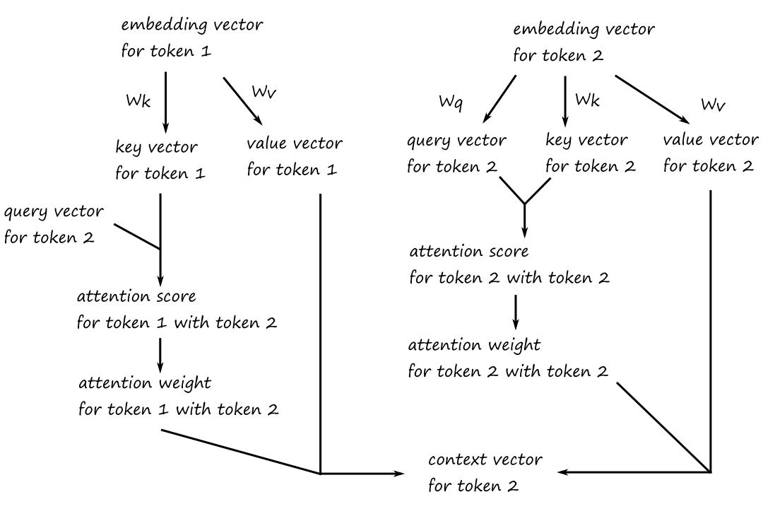
The idea behind calling them query vectors, key vectors, and value vectors can be loosely thought of as:
The word that we are calculating the attention score for is asking the other words if they are related to it (query vector), and the other words are responding (key vector) with how related they are to it (value vector).
The three weight matrices `W_q`, `W_k`, and `W_v` are randomly initialized. What makes them trainable is that their values are updated as the LLM learns more about what the words mean and how they're related to each other.
Casual Attention
A fast way to calculate the attention scores for all the words at once is to matrix multiply the word embedding vectors with themselves (in the simple self-attention case) or to matrix multiply the query vectors with the key vectors (in the regular self-attention case).
What we end up with is an attention weight matrix that could look something like this:
| The | chicken | didn't | cross | the | road | because | it | was | too | wide | |
| The | `0.06` | `0.09` | `0.08` | `0.10` | `0.07` | `0.11` | `0.10` | `0.07` | `0.08` | `0.12` | `0.12` |
| chicken | `0.11` | `0.05` | `0.09` | `0.08` | `0.10` | `0.07` | `0.09` | `0.10` | `0.07` | `0.12` | `0.12` |
| didn't | `0.08` | `0.12` | `0.04` | `0.13` | `0.09` | `0.08` | `0.07` | `0.09` | `0.07` | `0.11` | `0.12` |
| cross | `0.07` | `0.10` | `0.12` | `0.05` | `0.10` | `0.11` | `0.08` | `0.09` | `0.07` | `0.10` | `0.11` |
| the | `0.09` | `0.07` | `0.11` | `0.09` | `0.04` | `0.14` | `0.07` | `0.09` | `0.07` | `0.11` | `0.12` |
| road | `0.10` | `0.07` | `0.09` | `0.11` | `0.12` | `0.03` | `0.07` | `0.08` | `0.07` | `0.13` | `0.13` |
| because | `0.08` | `0.08` | `0.11` | `0.09` | `0.07` | `0.09` | `0.05` | `0.09` | `0.09` | `0.11` | `0.14` |
| it | `0.07` | `0.10` | `0.09` | `0.07` | `0.08` | `0.08` | `0.12` | `0.05` | `0.11` | `0.10` | `0.13` |
| was | `0.09` | `0.07` | `0.08` | `0.08` | `0.07` | `0.11` | `0.10` | `0.08` | `0.04` | `0.13` | `0.15` |
| too | `0.06` | `0.09` | `0.09` | `0.08` | `0.09` | `0.13` | `0.10` | `0.08` | `0.07` | `0.05` | `0.16` |
| wide | `0.07` | `0.08` | `0.10` | `0.09` | `0.08` | `0.11` | `0.09` | `0.09` | `0.09` | `0.10` | `0.10` |
The one problem with this is that this gives the LLM too much information. For example, let's say we wanted to predict what word would come after "road". In principle, we would make our prediction using only the words "The", "chicken", "didn't", "cross", and "the", i.e., the words that came before "road". But this attention matrix gives us information about words that come after "road".
Ideally, we would like to have something like this:
| The | chicken | didn't | cross | the | road | because | it | was | too | wide | |
| The | `1` | `0` | `0` | `0` | `0` | `0` | `0` | `0` | `0` | `0` | `0` |
| chicken | `0.49` | `0.51` | `0` | `0` | `0` | `0` | `0` | `0` | `0` | `0` | `0` |
| didn't | `0.22` | `0.27` | `0.51` | `0` | `0` | `0` | `0` | `0` | `0` | `0` | `0` |
| cross | `0.18` | `0.21` | `0.20` | `0.41` | `0` | `0` | `0` | `0` | `0` | `0` | `0` |
| the | `0.20` | `0.14` | `0.21` | `0.14` | `0.31` | `0` | `0` | `0` | `0` | `0` | `0` |
| road | `0.15` | `0.18` | `0.12` | `0.12` | `0.13` | `0.30` | `0` | `0` | `0` | `0` | `0` |
| because | `0.11` | `0.14` | `0.14` | `0.12` | `0.11` | `0.09` | `0.29` | `0` | `0` | `0` | `0` |
| it | `0.13` | `0.11` | `0.09` | `0.10` | `0.09` | `0.08` | `0.08` | `0.32` | `0` | `0` | `0` |
| was | `0.08` | `0.11` | `0.10` | `0.09` | `0.07` | `0.06` | `0.09` | `0.12` | `0.28` | `0` | `0` |
| too | `0.07` | `0.08` | `0.09` | `0.08` | `0.09` | `0.07` | `0.07` | `0.09` | `0.11` | `0.25` | `0` |
| wide | `0.05` | `0.07` | `0.08` | `0.09` | `0.08` | `0.06` | `0.08` | `0.10` | `0.09` | `0.10` | `0.20` |
The future tokens are "masked out" by applying what is called a casual attention mask.
An efficient way to achieve this is to set the attention scores above the diagonal to `-oo`, then normalize the matrix using softmax, which will turn the `-oo`s into `0`s (because `e^(-oo)` approaches `0`).
To prevent overfitting, a dropout mask can be further applied to the attention matrix. A dropout mask selects random attention weights to be "dropped" (turned into `0`s).
Multi-head Attention
Doing all of this with only one set of weight matrices `W_q`, `W_k`, `W_v` is implementing single-head attention. Doing all of this (in parallel) with multiple sets of weight matrices `W_q`, `W_k`, `W_v` is implementing multi-head attention.